Introduction

LiMA (liposome microarray-based assay) is a high throughput technology for monitoring the interaction of peripheral-membrane proteins with lipids. The core of LiMA lies in a chip comprising 120 unique liposomes coupled to high-content microscopy imaging allowing a quantitative and qualitative measurement (Saliba et al, 2014). The method has been recently applied (Vonkova et al, 2015) to study the recruitment mechanism of pleckstrin homology (PH) domains to distinct membranes. Since the method can generate thousands of interactions, bioinformatics methods are needed to enable data quality control. Along with an experimental protocol (Saliba et al, In revision), this webpage details the first steps of the data analysis. The provided pipelines will help to:
* (i) analyze the reproducibility of the measured interactions,
* (ii) check whether the liposome array contains obvious spatial bias,
* (iii) check whether the measured interactions are influenced by the protein concentration or the number of liposomes,
* (iv) extract a threshold to automatically classify interactions as binding or non-binding events.

Saliba, A.E., Vonkova, I, et al. (2014) A quantitative liposome microarray to systematically characterize protein-lipid interactions, Nature Methods, doi://10.1038/nature2734

Vonkova, I, Saliba, A.E., Deghou, S et al. (2015) Lipid Cooperativity as a General Membrane-Recruitment Principle for PH Domains Cell Reports, doi:10.1016/j.celrep.2015.07.054

The raw data used for this screen can be found at the following url:
http://vm-lux.embl.de/~deghou/data/ph-domain/

This tutorial illustrates the first step of the data analysis required in order to perform a sanity checkup of the readout `NBI`.

Datasets

Describe the dataset here
data = read.table("data-screen.tsv",header=T)

Technical Analysis Pipeline

The NBI can be in theory influenced by many parameters, like the protein concentration, the lipid concentration, the liposome array geometry etc
Therefore, it is necessary to conduct a sanity check up in order to identify any bias if there are any.

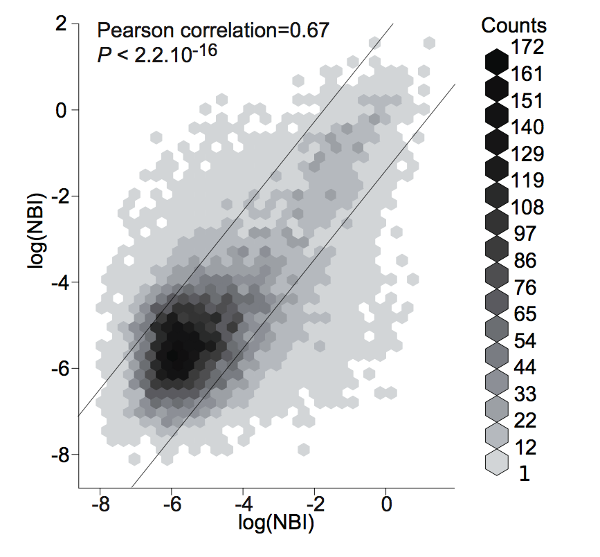
Reproducibility

  proteins = unique(as.character(data\$protein))
  lipids = unique(as.character(data$lipid))
  a = c()
  b = c()
  ind = 0
  color = ""
  for(prot in proteins){
    sub.p = subset(data,data$protein == prot)
    for(lip in lipids){
      sub = subset(sub.p,sub.p$lipid == lip)
      if(dim(sub)[1] != 0){
        replicates = sub\$signal.ratio
        lip.number = sub$liposome.number
        for(k in replicates){
          val1 = lip.number[which(replicates == k)]
          for(z in replicates[which(replicates == k) + 1:length(replicates)]){
            if(!is.na(k) & !is.na(z)){
              val2 = lip.number[which(replicates == z)]
              a[ind] = k
              b[ind] = z
              ind = ind + 1 
            }
          }
        } 
      }
    }
  }
  plot(a,b,log="xy")
  nbi_reproducibility = format(round(cor.test(df.rep\$a,df.rep\$b)$estimate, 3), nsmall=2)
  title = "NBI reproducibility (pearson coefficient) = "
  mtext(paste(title, nbi_reproducibility, sep=""),side=3)

Spatial bias

Quality-control is an important matter in the analysis of LiMA readout. One type of problem is regional bias, in which one region of a liposome array shows artifactually high or low NBIs. Current practice in quality assessment for microarrays does not address regional biases.

Coordinates file: coordinates.run.1.txt:
___________________________________________________________________________________________
1       2       3       4       5       6       7       8       9       10      11      12
13      14      15      16      17      18      19      20      21      22      23      24
25      26      27      28      29      30      31      32      33      34      35      36 
37      38      39      40      41      42      43      44      45      46      47      48  
49      50      51      52      53      54      55      56      57      58      59      60
61      62      63      64      65      66      67      68      69      70      71      72
73      74      75      76      77      78      79      80      81      82      83      84
85      86      87      88      89      90      91      92      93      94      95      96
97      98      99      100     101     102     103     104     105     106     107     108
109     110     111     112     113     114     115     116     117     118     119     120
___________________________________________________________________________________________

Processing code to visualize spatial bias:

  all = as.character(outer(seq(1,10),seq(1,12),paste))
  c.r.1 = read.table("coordinates.run.1.txt",sep='\t')
  c.r.2 = read.table("coordinates.run.2.txt",sep='\t')
  c.r.3 = read.table("coordinates.run.3.txt",sep='\t')
  c.r.4 = read.table("coordinates.run.4.txt",sep='\t')
  spatial.df = matrix(NA,ncol=12,nrow=10,dimnames=list(seq(1,10,1),seq(1,12,1)))  
  for(x in all){
    print(x)
    a = as.numeric(strsplit(x," ")[[1]][1])
    b = as.numeric(strsplit(x," ")[[1]][2])    
    lipids.round.1 = c(paste("lipid_id_",c.r.1[a,][b],sep=''))
    lipids.round.2 = c(paste("lipid_id_",c.r.2[a,][b],sep=''))
    lipids.round.3 = c(paste("lipid_id_",c.r.3[a,][b],sep=''))
    lipids.round.4 = c(paste("lipid_id_",c.r.4[a,][b],sep=''))
    lipids = unique(c(paste("lipid_id_",c.r.1[a,][b],sep=''),
paste("lipid_id_",c.r.2[a,][b],sep=''),
paste("lipid_id_",c.r.3[a,][b],sep=''),paste("lipid_id_",c.r.4[a,][b],sep='')))
    values = NULL
    if(round == "all"){
      print(lipids)
      values = data$signal.ratio[which(data$lipid %in% lipids)]  
    }else if(round == 1){
      values = data$signal.ratio[which(data$lipid %in% lipids.round.1)]  
    }else if(round == 2){
      values = data$signal.ratio[which(data$lipid %in% lipids.round.2)]  
    }else if(round == 3){
      values = data$signal.ratio[which(data$lipid %in% lipids.round.3)]  
    }else if(round == 4){
      values = data$signal.ratio[which(data$lipid %in% lipids.round.4)]        
    }
    v = mean(values,na.rm=TRUE)
    v = median(values,na.rm= TRUE)
    v = length(which(values > 0.037)) / length(values)
    spatial.df[a,][b] = v
  }  
  b = c(-1,0,0.05,0.1,0.15)
  b.number.of.bound.proteins = c(-1,0,60,120,180,300)
  bb = c(0,0.1,0.2,0.3,0.4,0.5)
  cc = c("white","#DBEBFF","#C3DBFA","#ACD0FE","#81B5FA")
  rownames(spatial.df)=c("A","B","C","D","E","F","G","H","I","J")
  spatial.df = spatial.df
  c = c(-10,-3.422,-2.09, -1.593,-1.117,-0.836)
  spatial.df = log(spatial.df)
  heatmap.2(spatial.df,trace="none",Rowv=NULL,Colv=NULL,
breaks=c(0,quantile(spatial.df,na.rm=TRUE)),col=cc,na.color="#81B5FA",key=FALSE)

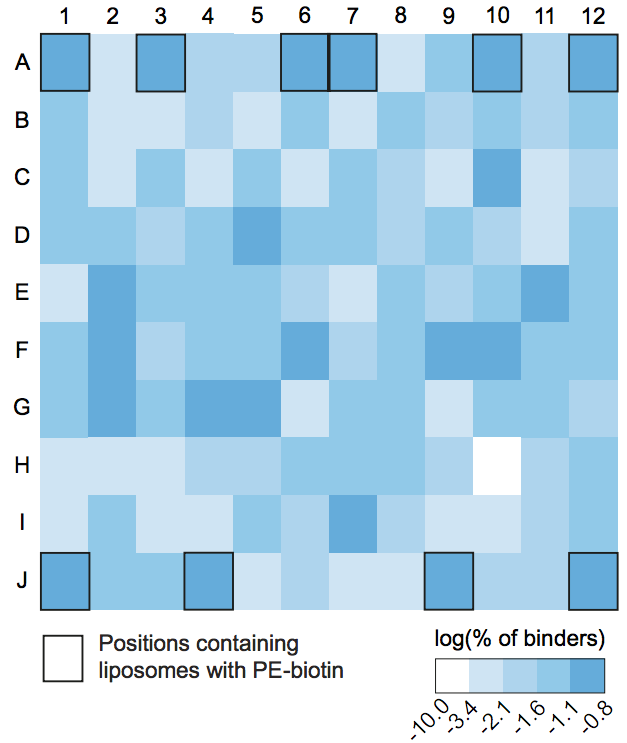plot Spatial bias plot

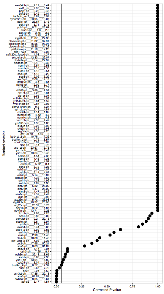
Concentration effects

Protein concentration effects

df = data.frame(protein = c(),conc.1 = c(),conc.2 = c(),p.value = c(),med.1=c())
proteins = unique(data$protein)
binding_threshold = 0.037
proteins.to.keep = proteins
a1 = c()
a2 = c()
a3 = c()
a4 = c()
a5 = c()
for(prot in proteins.to.keep){
  sub =  subset(data,subset = data$protein == prot & data$signal.ratio > binding_threshold)
  conc = unique(sub$protein.concentration)
  if(length(conc > 1)){
    v1 = sub\$signal.ratio[which(sub\$protein.concentration == conc[1])] 
    v2 = sub\$signal.ratio[which(sub\$protein.concentration == conc[2])] 
    v3 = sub\$signal.ratio[which(sub\$protein.concentration == conc[3])] 
    if(length(v1) > 1 & length(v2) > 1){
      p.t.test = t.test(v1,v2)$p.value
      w.t.test = wilcox.test(v1,v2)$p.value
      a1 = append(a1,prot)
      a2 = append(a2,conc[1])
      a3 = append(a3,conc[2])
      a4 = append(a4,p.t.test)
      a5 = append(a5,w.t.test)
      df = rbind(df,data.frame(protein = prot,
                               conc.1=conc[1],
                               conc.2 = conc[2],
                               p.value = p))
    }
    if(length(v1) > 1 & length(v3) > 1){
      p.t.test = t.test(v1,v3)$p.value
      w.t.test = wilcox.test(v1,v3)$p.value
      a1 = append(a1,prot)
      a2 = append(a2,conc[1])
      a3 = append(a3,conc[3])
      a4 = append(a4,p.t.test)
      a5 = append(a5,w.t.test)
      df = rbind(df,data.frame(protein = prot,
                               conc.1=conc[1],
                               conc.2 = conc[3],
                               p.value = p))
    }
    if(length(v2) > 1 & length(v3) > 1){
      p.t.test = t.test(v2,v2)$p.value
      w.t.test = wilcox.test(v2,v3)$p.value
      a1 = append(a1,prot)
      a2 = append(a2,conc[2])
      a3 = append(a3,conc[3])
      a4 = append(a4,p.t.test)
      a5 = append(a5,w.t.test)
      df = rbind(df,data.frame(protein = prot,
                               conc.1=conc[2],
                               conc.2 = conc[3],
                               p.value = p))
    } 
  }
}
dpc = data.frame("prot" = a1,
                 "conc_1" = a2,
                 "conc_2" = a3,
                 "p.value.t.test" = a4,
                 "w.value.t.test" = a5,
                 "w.corrected" = p.adjust(a5,'hochberg'),
                 "label" = paste(a1,a2,a3,sep='___'))
dpc = dpc[order(dpc\$w.corrected),]
dpc\$label = as.character(dpc\$label)
dpc\$label = factor(dpc\$label,dpc\$label)
plot = ggplot(dpc,aes(x = factor(label),y = w.corrected))
plot = plot + geom_point(size = 5) + coord_flip()
plot = plot + geom_hline(yintercept = 0.05) + theme_bw() 
plot = plot + ylab("Corrected P value") + xlab("Ranked proteins")

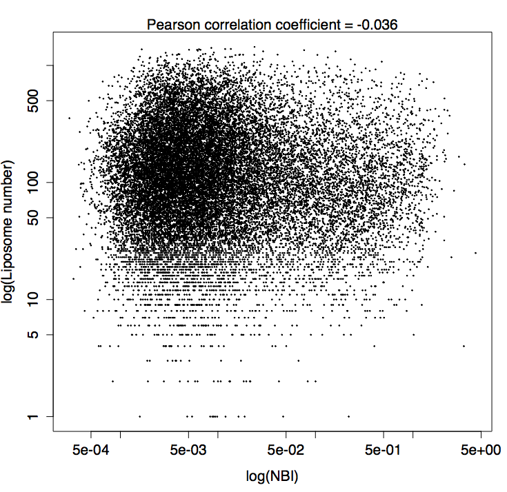
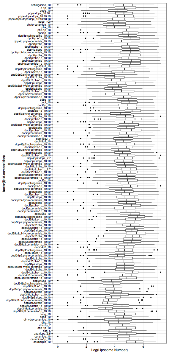
Liposome number

pearson_cor = cor.test(data\$signal.ratio,data\$liposome.number)\$estimate
pearson_cor = format(round(pearson_cor,3),nsmall=2),sep="")
plot(data\$signal.ratio,data\$liposome.number,
cex=0.2,
log="xy",
xlab = "log(NBI)",
ylab = "log(Liposome number)")
mtext(paste("Pearson correlation coefficient = ",pearson_cor,side=3)

liposome_composition = data\$lipid.composition
liposome_number = data\$liposome.number
plot = ggplot(data,aes(x = factor(lipid.composition),y = log(liposome.number)))
plot = plot + geom_boxplot() + theme_bw()

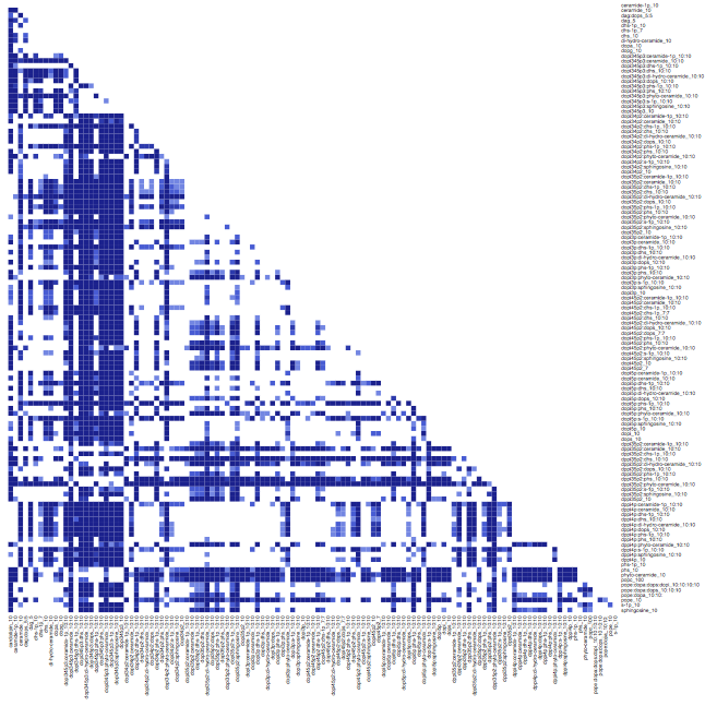
res.p.val = pairwise.wilcox.test(liposome_number,liposome_composition)
heatmap.2(res.p.val\$p.value,trace="none",breaks=c(0,0.0001,0.001,0.01,0.1,1),
col=c("#072B8E","#1C43AE","#3A64D5","#6B8BE4","#FFFFFF"),
Rowv=FALSE,Colv=FALSE,key=FALSE,margins=c(20,20))

Threshold extraction

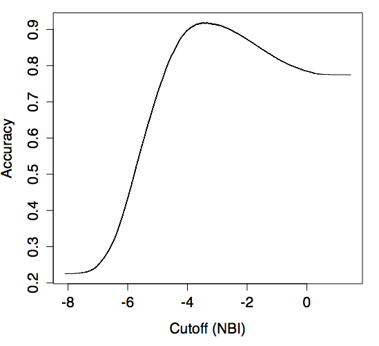
Making use of the manual annotation, one can run a classifier in order to extract a threshold that can be used for the rest of the analysis as interaction predictor. The threshold can be manually extracted, or following one of the two proposed methods, namely, by maximixing the accuracy or by minimizing the sum of the sensitivity and specificity.

Maximizing accuracy

data = data[data\$man.annotation != 0,]
predClass = prediction(log(data\$signal.ratio),data\$man.annotation)
BMacc <- performance(predClass, measure="acc")
plot(BMacc,xlab="Cutoff (NBI)")
MaxAcc <- max(BMacc@y.values[[1]])
UnlistXacc <- unlist(BMacc@x.values[[1]])
CutoffAcc <- UnlistXacc[which.max(BMacc@y.values[[1]])]
threshold_by_maximization_of_accuracy = exp(CutoffAcc)

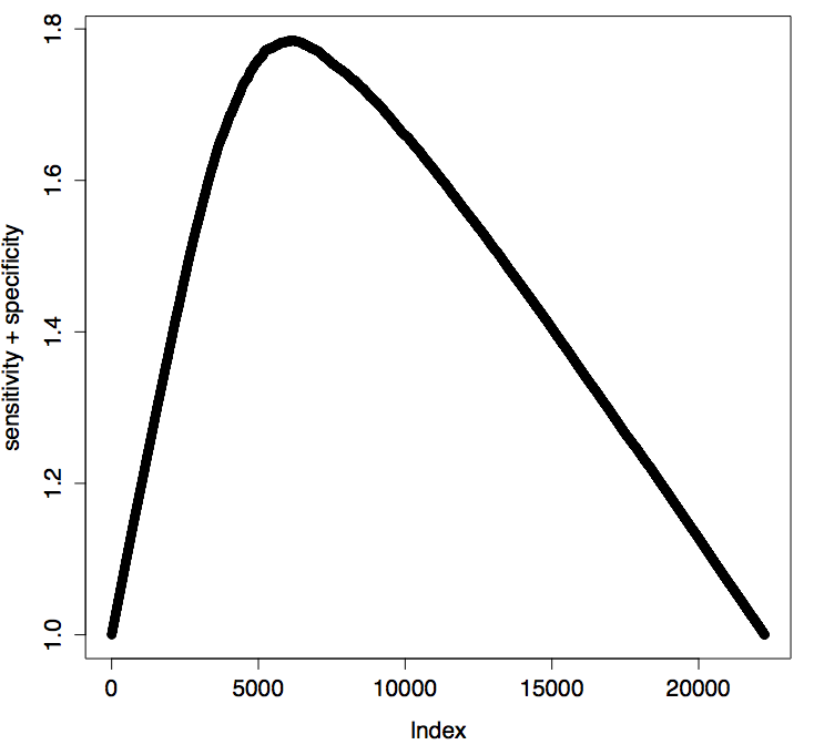
Sensitivity + Specificity minimization

data = data[data\$man.annotation != 0,]
prefClass = performance(prediction(log(data\$signal.ratio),data\$man.annotation),'tpr','fpr')
fpr <- prefClass@x.values[[1]]
tpr <- prefClass@y.values[[1]]
sum <- tpr + (1-fpr)
plot(sum,ylab = "sensitivity + specificity")
index <- which.max(sum)
threshold_by_minimization_of_sensitivity_specificity <- prefClass@alpha.values[[1]][[index]]

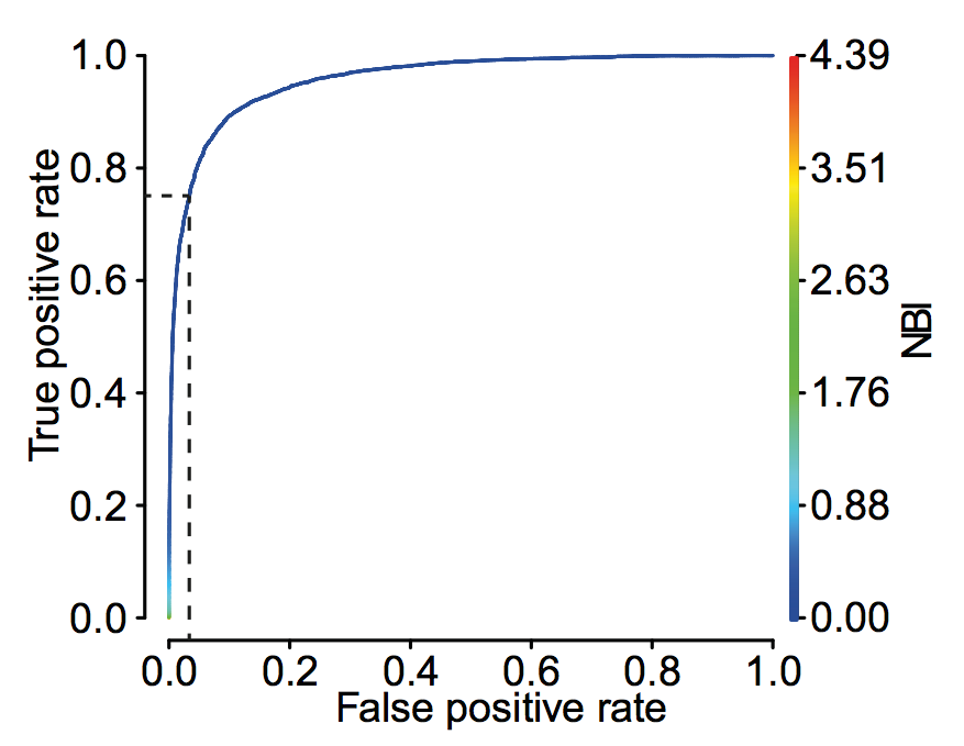
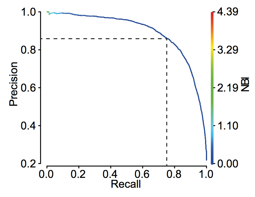
ROC curve and precision recall curve

data = data[data\$man.annotation != "0",]
a = data\$signal.ratio[data\$protein == prot]
b = data\$man.annotation[data\$protein == prot]
roc_curve = performance(prediction(a,b),"tpr","fpr")
auc = performance(prediction(a,b),"auc")
prec_rec = performance(prediction(a,b),"prec","rec")
auc = performance(prediction(a,b),"auc")@y.values[[1]]
plot(roc_curve)
plot(prec_rec)