- Using SMASH
- Real sample from planet Earth
- Preparing SMASH for the metagenome
- Loading the metagenome into SMASH
- Assembling the metagenome
- Predicting protein coding genes
- Hypothetical sample from planet X
- Phylogenetic annotation of samples
- Functional annotation of proteins
- Comparative analysis of metagenomes
Using SMASH
There are several scripts that provide the interface to the SMASH Perl modules. These scripts are located in the bin directory of the SMASH installation. A normal user does not need to know the structure of the Perl modules - not even where they are and what they do. For expert users who need to use them, or just know them, we recommend reading the "Programmers Manual". In this section, we walk you through the analysis of a metagenomics sample, when all you have are the raw data.
Real sample from planet Earth
First we use a very simple example of a simple microbial community. For this, we use the Acid Mine Drainage sample used in Tyson et al, 2004. Download the raw data files from "download examples" in downloads page. To analyze this data, we would use the Celera assembler to assemble and GeneMark to predict genes.
Preparing SMASH for the metagenome
Let us now add a new collection for multiple metagenomes that we would analyze.
        addMetaGenomeCollection.pl --title=Pub2008 \
                --description="Collection of metagenomes published before 2008"
If this succeeds, you will see a message that ends with:
        <output>MC1</output>
        ********************************************************
          Metagenome collection MC1 added to SMASH
        ********************************************************
The <output> XML tag is for parsing the output of the SMASH scripts in an automated pipeline. For more details, see addMetaGenomeCollection.pl. Now let us add a metagenome for the AMD dataset. Assuming that the collection was MC1 (change it to the actual id you receive from the script), run the following command:
        addMetaGenome.pl --collection=MC1 --title=AMD \
                --description="Acid Mine Drainage data from Tyson et al, 2004"
If this succeeds, you will see a message such as:
        <output>MC1.MG1</output>
        ********************************************************
          Metagenome MC1.MG1 added to MC1
        ********************************************************
Loading the metagenome into SMASH
Let us add the data to SMASH. Assuming that the new metagenome was called MC1.MG1, run the following command:
        loadMetaGenome.pl --metagenome=MC1.MG1 --sample "Iron Mountain" --type=sanger \
                --reads examples/AMD.fasta --quals examples/AMD.qual \
                --xmls examples/AMD.xml \
                --weird_fasta
loadMetaGenome.pl is a very powerful script with numerous options that help you customize loading your data. For example, if the sequence trimming software lucy was installed with Smash (using --enable-lucy=yes, which is the default), you could add --quality_trim=lucy to quality trim the sequences. For more details, see loadMetaGenome.pl. The output looks like this (with the --quality_trim=lucy option):
        Reading fasta files ... done
        Reading traceinfo xml files: processing traces (counts in 10000) .........10.. done (Processed 124805 traces.)
        Generating remapped fasta file ... done
        Generating remapped qual file ... done
        Generating remapped xml file ... done
        Trimming reads for low quality sequences .....lucy: Warning! No vector file given; vector removal will not be done!
        lucy: Warning! No splice file given; splice site will not be trimmed!
        . done
        Making list of reads that remain ... done
        Removing completely trimmed reads ... done
        Generating new xml file for the trimmed reads ... done
        Loading read information into database ... done
        <output>success</output>
        ********************************************************
          Metagenome MC1.MG1 loaded to SMASH
        ********************************************************
Assembling the metagenome
Now let us assemble this metagenome. We need an assembler for this purpose, and we will use Celera for this example.
        doAssembly.pl --metagenome=MC1.MG1 --assembler=Celera --version=6.1 \
                --genome_size=15000000
When this process finishes successfully, you will see an output like this:
        <output>MC1.MG1.AS1</output>
        ********************************************************
          Assembly id assigned for this assembly: MC1.MG1.AS1
        ********************************************************
In this example, the --version=6.1 argument is optional, if that is the only version installed, e.g., using
./configure --enable-celera
For more details, see doAssembly.pl. Now that this has finished successfully, let us load the assembly into SMASH. We do that using:
loadAssembly.pl --assembly=MC1.MG1.AS1
The progress of this process looks like this:
        Contig2Read:
                Reading GFF file ... done
                Loading into database .... done
        Scaf2Contig:
                Reading GFF file ... done
                Loading into database .... done
        <output>success</output>
        ********************************************************
          Assembly MC1.MG1.AS1 loaded to SMASH
        ********************************************************
For more details, see loadAssembly.pl.
Predicting protein coding genes
Now that we have the assembly in the database, we are ready to predict protein coding genes in the assembly. The following command uses GeneMark to predict genes:
        doGenePrediction.pl --assembly=MC1.MG1.AS1 --predictor=GeneMark \
                --version=2.6p --self_train
This will run on a single cpu of the execution host. Since metagenome assemblies are very big, gene prediction can take a long time. Please see doGenePrediction.pl for ways to parallelize it and reduce the run-time. This invocation will report the id assigned for this gene prediction run.
        <output>MC1.MG1.AS1.GP1</output>
        ********************************************************
          Prediction id assigned for this gene set: MC1.MG1.AS1
        ********************************************************
For more details, see doGenePrediction.pl. When gene prediction is finished, we are ready to load the genes into the SMASH database using the following command:
loadGenePrediction.pl --genepred=MC1.MG1.AS1.GP1
When this finishes successfully, you would see the following output:
        <output>success</output>
        ********************************************************
          Gene prediction MC1.MG1.AS1.GP1 loaded to SMASH
        ********************************************************
Please see loadGenePrediction.pl for detailed information.
Hypothetical sample from planet X
For the purposes of this walkthrough, we assume a hypothetical metagenome sample obtained from planet X. Since this is part of a bigger extra-terrestrial study, we need a metagenome collection for this and future extra-terrestrial projects. Two samples were collected from planet X at two different time-points A and B. Both of these samples were sequenced using Sanger and 454 Titanium technologies. In this example, we want to consider these two timepoints as a single metagenome - we will assemble them together and analyze them together. Therefore they are loaded as two samples from the same metagenome. If we wanted to analyze them separately, we would add them as two different metagenomes (See "Metagenome data").
Raw data
Raw data is the term we use loosely for all sequence data associated with a metagenome sample. To make the most of SMASH and its analysis scripts, we recommend that you record as much metadata as possible, and store them in the database as well.
- Sanger data
- Sanger sequencing usually produces chromatogram/trace files and the sequencing centers then generate sequence and quality files for them. SMASH requires the sequence and quality files in FASTA format along with the sequence metadata in Trace Archive XML format (http://www.ncbi.nlm.nih.gov/Traces/trace.cgi?cmd=show&f=rfc&m=doc&s=rfc). Sequence metadata are necessary for assembling the reads from the sample.
- 454 Titanium data
- 454 Titanium sequencing produces flowgrams (dumped into sff files) and there are several tools to extract the sequences from these sff files. The sequencing facility will also be able to provide you the sequences in FASTA format. SMASH normally requires the sequence and quality files in FASTA format. However, if you have configured a version of Celera assembler in SMASH, you can let SMASH convert the SFF files to FASTA format using the sffToCA utility part of the Celera assembler. This option is highly recommended if you are planning to use the Celera assembler.
Preparing raw data
Raw data needs to be cleaned up before it is loaded into SMASH repository. Cleaning up involves removing the vector/adapter sequences, low quality ends of sequence reads and some project specific screening. For example, in Human Gut Microbiome projects, we routinely filter out reads that match the human genome since there could be some human DNA in the stool samples. SMASH assists you in screening vector/adapter sequences using lucy (http://lucy.sourceforge.net/) or Forge when you load the sequences into the database. Project specific screening of sequences must be done by the user beforehand, and vector/adapter screening can also be done by the user.
Loading raw data
- NOTE
- For the sake of brevity and clarity, I have dropped the location of the scripts in the following command snippets. This will be fine if the bin directory of the SMASH installation is in you
$PATHenvironment variable. Otherwise, be sure to use the full path of each perl script.
Once you have the screened/clean raw data, you are ready to load them in the repository.
Since this is the first sample in the extra-terrestrial study, we must first add a metagenome collection for this sample. This is done as follows:
        addMetaGenomeCollection.pl --title "E.T." \
                --description "Extra-terrestrial metagenomes"
We now add this planet X metagenome to the E.T. metagenome collection.
        addMetaGenome.pl --collection "MC1" --title "planetX" \
                --description "Metagenome sample from planet X; Date:20090909; Coordinates:30.5,70.3,24.5,109.2; Temperature:27C"
Assuming we have done the cleaning/screening steps, deposit the sequence data into the repository.
        loadMetaGenome.pl --metagenome=MC1.MG1 --sample "time A" --type=sanger \
                --reads timeA.fasta --quals timeA.qual --xmls timeA.xml
        loadMetaGenome.pl --metagenome=MC1.MG1 --sample "time B" --type=sanger \
                --reads timeB.fasta --quals timeB.qual --xmls timeB.xml
        loadMetaGenome.pl --metagenome=MC1.MG1 --sample "time A" --type=454 \
                --library libA --reads flowgramA.fasta --quals flowgramA.qual
        loadMetaGenome.pl --metagenome=MC1.MG1 --sample "time B" --type=454 \
                --library libB --reads flowgramB.fasta --quals flowgramB.qual
Note that the last two lines assume that you have generated FASTA files containing the DNA sequences and the corresponding quality sequences. These files are usually created by the software bundled with Roche 454 instruments and will be named 454Reads.fna and 454Reads.qual. If you want to directly upload the sequences from the SFF files (flowgrams) from the Roche 454 instruments, SMASH needs the SFF file reader bundled with the Celera assembler. If you have the Celera assembler installed and configured in SMASH, the last two lines could be replaced by
        loadMetaGenome.pl --metagenome=MC1.MG1 --sample "time A" --type=454 \
                --library timeA --sffs flowgramA.sff
        loadMetaGenome.pl --metagenome=MC1.MG1 --sample "time B" --type=454 \
                --library timeB --sffs flowgramB.sff
Please see loadMetaGenome.pl for detailed information.
Assembly
Since we have a mixture of Sanger and 454 Titanium sequences, we are now limited to using the Celera assembler. In this case, we would invoke the assembly as follows:
doAssembly.pl --metagenome=MC1.MG1 --assembler=Celera
This processes the final outputs of Celera assembler and converts them to SMASH format. Please see doAssembly.pl for detailed information. We are now ready to load this assembly into the SMASH database using the following command:
loadAssembly.pl --assembly=MC1.MG1.AS1
Please see "Assembling the metagenome" for detailed information.
Gene Prediction
The following command uses GeneMark to predict genes:
        doGenePrediction.pl --assembly=MC1.MG1.AS1 --predictor=GeneMark \
                --version=2.6p --self_train
and the next one will load them into SMASH:
loadGenePrediction.pl --genepred=MC1.MG1.AS1.GP1
Please see "Predicting protein coding genes" for detailed information.
Phylogenetic annotation of samples
Reads from metagenomic samples can be assigned to a reference species through BLAST based sequence similarity. We use blastn to align the reads to the reference genome set. For more details on how to perform this, and to analyze the phylogenetic composition of the samples, please see "Phylogenetic annotation of samples".
Functional annotation of proteins
Predicted genes are assigned to orthologous groups using BLAST based sequence homology to known proteins. We use the eggNOG orthologous groups to assign functions to predicted genes. First of all, genes need to be blastp'ed against the set of eggNOG proteins. Then they can be mapped to orthologous groups. For more details, see "Functional annotation".
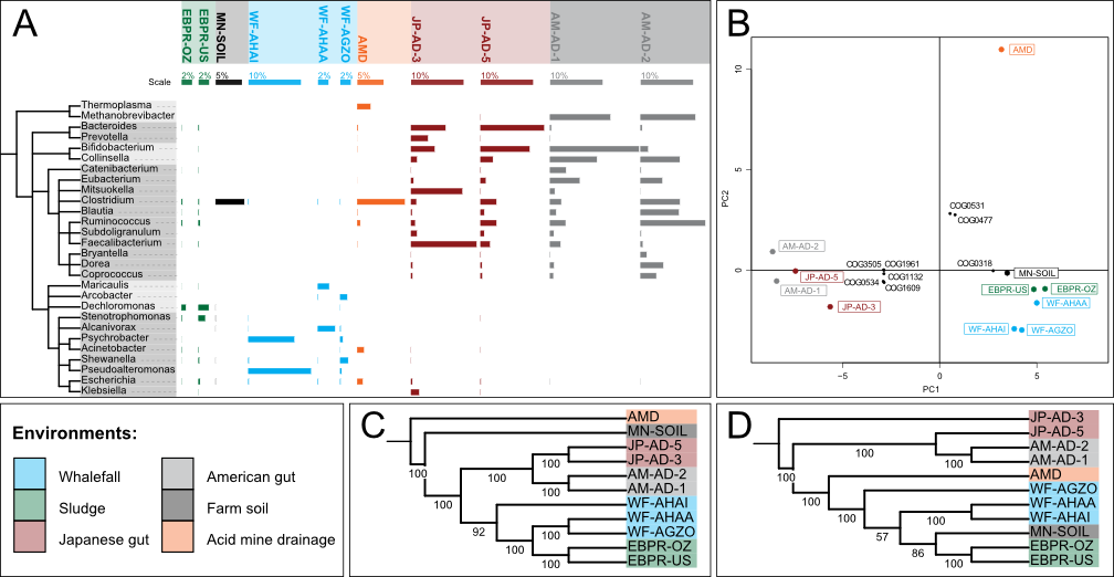
Comparative analysis of metagenomes
Once you have phylogenetically or functionally annotated your metagenomes, you can start comparing them based on the phylogenetic or functional composition. For more details, see "Comparative metagenomic analysis".