- Comparative metagenomic analysis
- 1. Phylogenetic analysis using reference genome mapping
- 1.1. Parse the BLAST output
- 1.2. Summarize phylogenetic composition
- 1.3. Cluster samples without bootstrapping
- 1.4. Cluster samples with bootstrapping
- 1.5. Display the phylogenetic composition on iTOL
- 2. Functional analysis using eggNOG mapping
Comparative metagenomic analysis
Currently,
three types of comparative analysis are possible - two phylogenetic and one functional analyses.
All three types of comparative analyses are performed by a script that is my personal favorite - doComparativeAnalysis.pl.
This script takes the analysis type through --analysis argument and processes the data accordingly.
The information on the samples that are being compared is provided through --list option - this is a file containing one metagenome/gene-prediction id per line.
1. Phylogenetic analysis using reference genome mapping
This is the most sensitive phylogenetic analysis for a metagenome sample provided of course that the species population has relatives in the reference genome set. The following are the prerequisites before running this analysis:
- 1. Sample information
- For example, if your list file contains
MC20.MG1 MC20.MG2 MC30.MG5- then these three metagenomes must have been added using addMetaGenome.pl, reads must have been loaded into SMASH using loadMetaGenome.pl, and updateStats.pl must have been run for MC20 and NC30 after these three metagenomes have been loaded. If you are not sure, then you should run
updateStats.pl --collection=MC20 --upto=reads updateStats.pl --collection=MC30 --upto=reads- This will summarize the number of reads, inserts, etc for each metagenome in a summary table that doComparativeAnalysis.pl will query later. The script will also retrieve sample labels from the database.
- 2. You have a set of reference genome sequences.
- These could be WGS scaffolds, contigs, or complete genomes. Please do not use a set of WGS reads since this will mess up genome size calculations. If you enabled refgenome-db by specifying
--enable-refgenomedbto theconfigurescript during installation, SMASH will automatically download a reference genome sequence database for you. The latest reference set in SMASH is called reference_genomes.20100704.- 3. You have the taxonomical information of these.
- Either these are available in the
RefOrganismDBdatabase in SMASH, or you have a flat file downloaded from http://www.bork.embl.de/software/smash/downloads/reference_genomes/. If you make your own reference genome database, you could make this file yourself: please check the header (first line) of the file for which fields contain what information.- 4. Reads have been BLASTed against the reference genome sequences.
- The output of this BLAST run must be MC20.MG1.reference_genomes.20100704.blastn in the analyses directory for MC20.MG1.
We are now ready to run the comparative phylogenetic analysis. Here are the steps to do this.
1.1. Parse the BLAST output
The first step is to parse the BLAST outputs. You can do this by running:
        doComparativeAnalysis.pl --analysis=refgenome --list=list.txt \
                --refdb=reference_genomes.20100704 --tag=trial1 \
                --identity=85 --normalize=data \
                --mode=raw
This will produce the file trial1.feature_vector.rawcount.refgenome.reference_genomes.20100704. This file is in
Rtable format, containing NCBI taxonomy ids as rows and samples (in this case just MC20.MG1) as columns. It could look like:MC20.MG1 MC20.MG2 MC30.MG5 -1 489 387 899 435590 1338 994 1232 272559 839 789 403 537011 241 358 491which means that, for sample MC20.MG1, out of 2907 reads, 489 (17%) of the reads could not be mapped at all (that's what -1 means), 46% of the reads were mapped to Bacteroides vulgatus ATCC 8482 (taxonomy id 435590), 29% of the reads to Bacteroides fragilis NCTC 9343 (taxonomy id 272559) and 8% of the reads were mapped to Prevotella copri DSM 18205 (taxonomy id 537011), all above the sequence identity threshold of 85%.
Once we have parsed the BLAST files and created the file above, there are several things we could do.
1.2. Summarize phylogenetic composition
To obtain a summary of the phylogenetic composition of samples at any taxonomic rank, you can run:
        doComparativeAnalysis.pl --analysis=refgenome --list=list.txt \
                --refdb=reference_genomes.20100704 --tag=trial1 \
                --level=genus --identity=85 --normalize=data \
                --mode=summary
The above command generates a normalized genus level relative abundance distribution like this:
        MC20.MG1        MC20.MG2        MC30.MG5
        -1      0.21949439      0.19564004      0.35539844
        Bacteroides     0.66766555      0.61557832      0.44212809
        Prevotella      0.11284007      0.18878164      0.20247347
in the file trial1.feature_vector.summary.refgenome.genus.reference_genomes.20100704. Note here that the percentage of each genus does not match the percentage of reads mentioned earlier, since the summary is made after correcting for genome size. For example, unknown fraction changed from 17% to 22%, Prevotella from 8% to 11.3%, Bacteroides from 76% to 66.7%.
1.3. Cluster samples without bootstrapping
Clustering samples involves the following two steps.
1.3a. Estimate inter-sample distances
Since this threshold is suitable for genus level mapping, we will now create the genus abundance of this sample.
        doComparativeAnalysis.pl --analysis=refgenome --list=list.txt \
                --refdb=reference_genomes.20100704 --tag=trial1 \
                --level=genus --identity=85 --normalize=data \
                --mode=distmat
This will generate a normalized genus level abundance profile. These numbers are generated after two steps. First the number of reads mapping to each genome is normalized by the genome length. Then these normalized values are added according to the genus, where 816 and 838 are the NCBI taxonomy ids of Bacteroides and Prevotella, respectively. The abundances of all genomes belonging to Bacteroides have been summed together into the abundance of Bacteroides. This resides in a file trial1.feature_vector.rawcount.refgenome.genus.reference_genomes.20100704. This profile is used to generate a normalized genus level relative abundance distribution like this:
        MC20.MG1        MC20.MG2        MC30.MG5
        -1      0.21949439      0.19564004      0.35539844
        816     0.66766555      0.61557832      0.44212809
        838     0.11284007      0.18878164      0.20247347
in the file trial1.feature_vector.jsd.refgenome.genus.reference_genomes.20100704.
This abundance distribution is then used to make a distance matrix in phylip format:
        3
        MC20.MG1   0.000000 0.075521 0.161573
        MC20.MG2   0.075521 0.000000 0.137878
        MC30.MG5   0.161573 0.137878 0.000000
in the file trial1.distance.jsd.refgenome.genus.reference_genomes.20100704.
1.3b. Cluster using these distances
If you want to cluster these samples using this distance matrix, then run this:
        doComparativeAnalysis.pl --analysis=refgenome --list=list.txt \
                --refdb=reference_genomes.20100704 --tag=trial1 \
                --level=genus --identity=85 --normalize=data \
                --mode=cluster
This will use
neighbormethod from thephylippackage to cluster these samples, and upload this tree to the iTOL website.
1.4. Cluster samples with bootstrapping
Clustering with bootstrap support requires the following two steps.
1.4a. Estimate inter-sample distances
If you run, instead
        doComparativeAnalysis.pl --analysis=refgenome --list=list.txt \
                --refdb=reference_genomes.20100704 --tag=trial1 \
                --level=genus --identity=85 --normalize=data \
                --mode=bootstrap+distmat
this will make 100 bootstrap replicates from the input file, and create a distance matrix as mentioned above for each replicate.
1.4b. Cluster using these distance
If you want to cluster these samples with bootstrap support, then run this:
        doComparativeAnalysis.pl --analysis=refgenome --list=list.txt \
                --refdb=reference_genomes.20100704 --tag=trial1 \
                --level=genus --identity=85 --normalize=data \
                --mode=bootstrap+cluster
This will read all the 100 distance matrices, use the
neighborprogram to make 100 trees and then use theconsenseprogram to produce a consensus tree with bootstrap support, which will be loaded to iTOL.
1.5. Display the phylogenetic composition on iTOL
If you would like to display the genus distribution as graphs using iTOL, you can upload this to the iTOL server by running the following command:
        doComparativeAnalysis.pl --analysis=refgenome --list=list.txt \
                --refdb=reference_genomes.20100704 --tag=trial1 \
                --level=genus --identity=85 --normalize=data \
                --mode=itol
A successful run looks like this:
        Avg. genome size = 3538803
        Processing samples ... done
        Filtering samples ... done
        Running: /usr/bin/perl /usr/local/Smash/bin/iTOL_uploader.pl --config trial1.refgenome.cfg
        ITOL:
        ITOL: iTOL batch uploader
        ITOL: ===================
        ITOL: Upload successful. Your tree is accessible using the following iTOL tree ID:
        ITOL:
        ITOL: 111111111111111111111111
        ITOL:
        Upload successful. You can view this tree on iTOL using this URL:
        http://itol.embl.de/external.cgi?tree=111111111111111111111111
        Running: /usr/bin/perl /usr/local/Smash/bin/iTOL_downloader.pl --tree 1111111111111111111
        1111 --format svg --outputFile trial1.refgenome.downloaded.svg --fontSize 20 --displayMod
        e normal --colorBranches 1 --alignLabels 1 --scaleFactor 1 --showBS 1 --BSdisplayValue M0
        --BSdisplayType text --datasetList dataset1

        iTOL batch downloader
        =====================
        Exported tree saved to trial1.refgenome.downloaded.svg
The script tells you the commands it is executing to upload and download the tree to iTOL. Lines beginning with
"ITOL:"are what it received as a response from iTOL webserver, for your information. When the upload is successful, you can view the tree following the link provided. Hovering over any bar will show the name of the dataset, and the abundance of the corresponding genus in that dataset.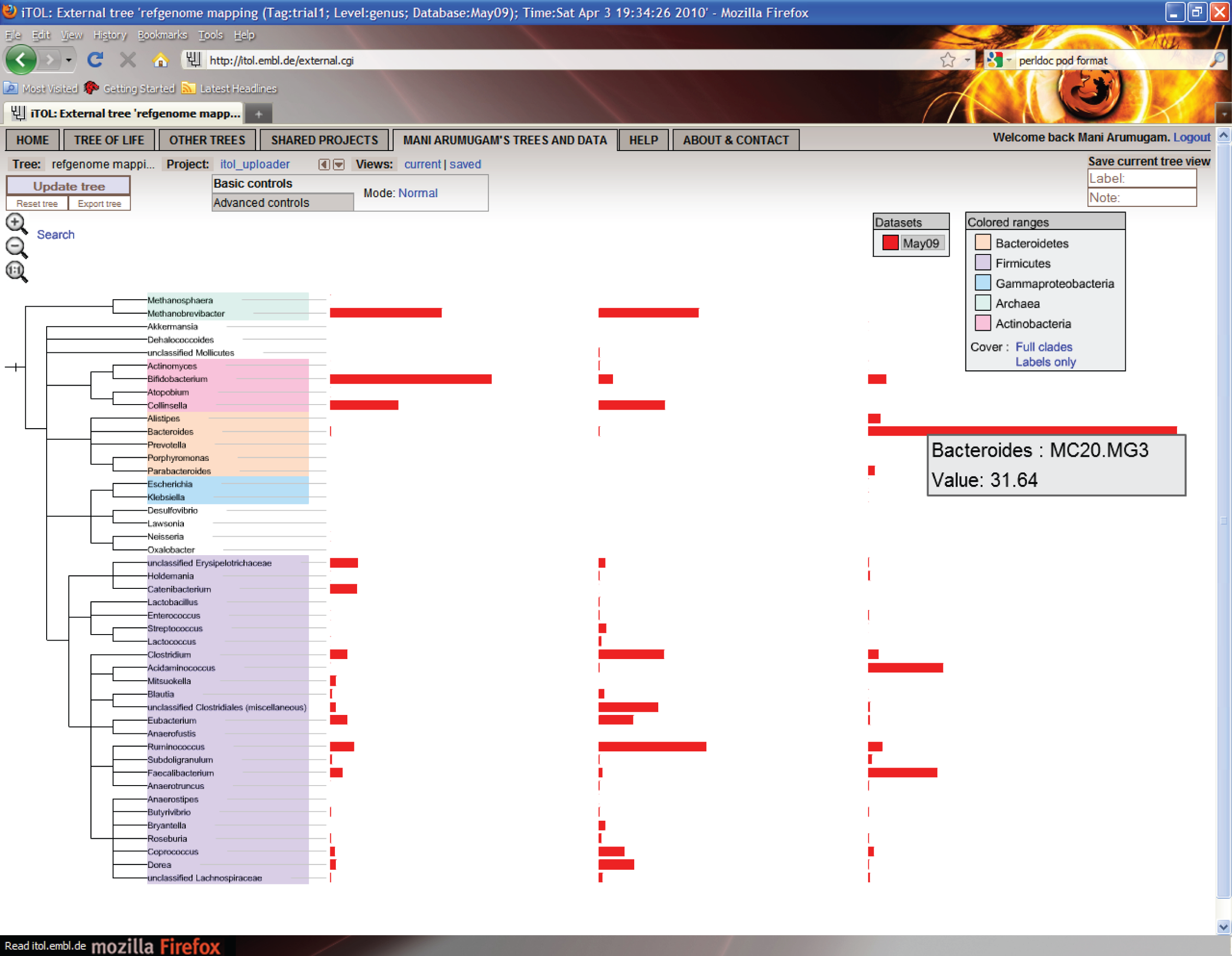
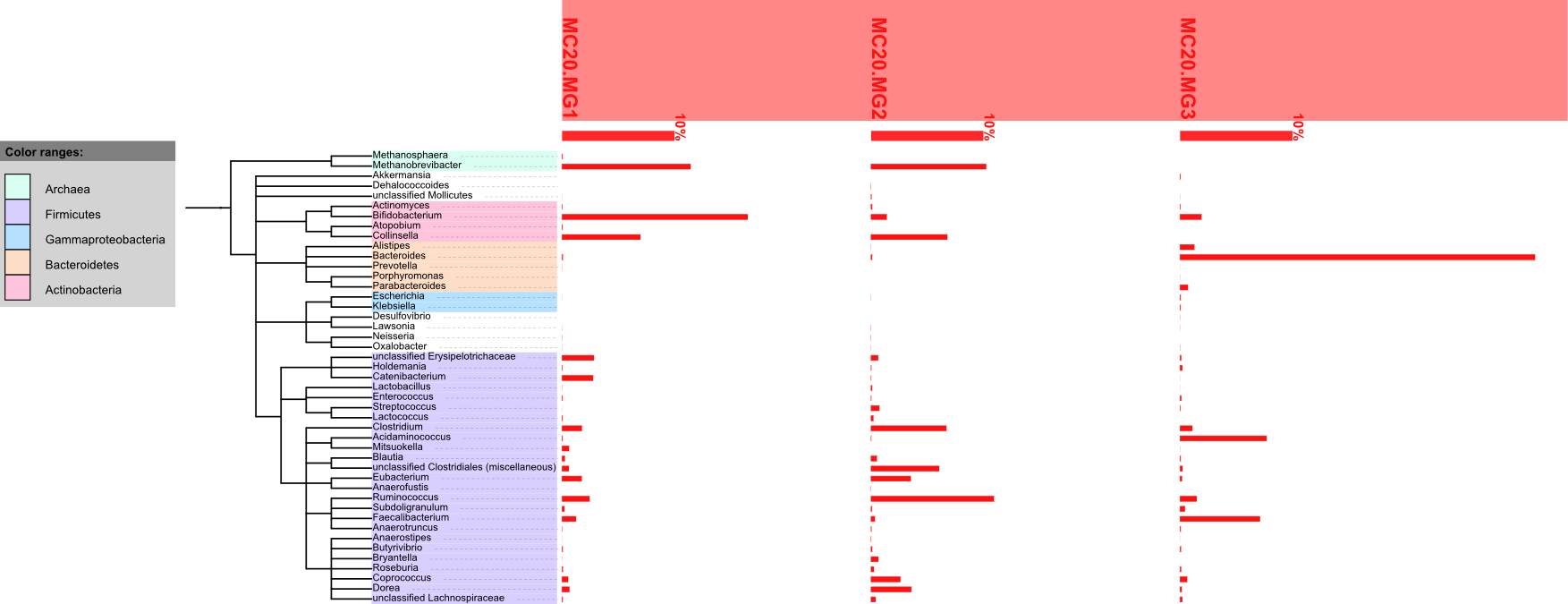
You can also use the SVG file listed in the last line for the tree that contains additional label information.
2. Functional analysis using eggNOG mapping
The following are the prerequisites before running this analysis:
- 1. Sample information
- For example, if your list file contains
MC20.MG1.AS1.GP1 MC20.MG2.AS1.GP1 MC30.MG5.AS1.GP1- then these three gene predictions must have been loaded using loadGenePrediction.pl, and updateStats.pl must have been run for MC20 and NC30 after these three metagenomes have been loaded. If you are not sure, then you should run
updateStats.pl --collection=MC20 --upto=genes updateStats.pl --collection=MC30 --upto=genes- This will summarize the number of genes and estimate the read coverage for each gene in the gene prediction in a summary table that doComparativeAnalysis.pl will query later. The script will also retrieve sample labels from the database.
- 2. Predicted proteins have been BLASTed against the eggNOG database
- The output of this BLAST run must be, for example, MC20.MG1.AS1.GP1.eggnog2.blastp in the gene_pred directory for MC20.MG1.AS1.GP1.
- 3. Predicted proteins have been annotated using
doOrthologMapping.pl- The output of this annotation run must be, for example, MC20.MG1.AS1.GP1.eggnogmapping.txt in the gene_pred directory for MC20.MG1.AS1.GP1.
We are now ready to run the comparative functional analysis.
2.1. Parse the eggNOG mapping output
The first step is to parse the eggnog mapping outputs by running
        doComparativeAnalysis.pl --analysis=functional --list=list.txt \
                --refdb=eggnog --tag=trial1 \
                --level=og --normalize=hits \
                --mode=raw
This will produce the file trial1.feature_vector.rawcount.functional.eggnog. This file is in
Rtable format, containing eggNOG orthologous group id's as rows and samples (in this case just MC20.MG1.AS1.GP1 etc) as columns. It could look like (only top 10 lines shown):SampleXY SampleYZ SampleAB COG0014 24.90619625 25.09718986 24.90619625 COG0016 6.37547157 5.95759717 5.95759717 COG0022 7.18813387 7.18813387 7.18813387 COG0055 10 10 9.55326460 COG0056 11.34920635 11.34920635 1.37522769 COG0057 9.43329925 9.57109873 9.33395946 COG0072 6.93965517 6.93965517 6.93965517 COG0095 0 11.82809224 0 COG0115 6.71621622 6.71621622 6.71621622which means that, sample SampleXY contains 24.9 functional units of COG0014, 6.4 functional units of COG0016, etc. These numbers are not comparable across samples yet, since these have not been normalized for sample size.
Once we have parsed the mapping files and created the file above, there are several things we could do.
2.2. Summarize functional composition
To obtain a summary of the functional composition of samples, you can run:
        doComparativeAnalysis.pl --analysis=functional --list=list.txt \
                --refdb=eggnog --tag=trial1 \
                --level=og --normalize=hits \
                --mode=summary
The above command generates a normalized OG level relative abundance distribution like this:
        SampleXY        SampleYZ        SampleAB
        COG0014__Gamma-glutamyl_phosphate_reductase                             0.01360761      0.01382180      0.01357623
        COG0016__Phenylalanyl-tRNA_synthetase_alpha_subunit                     0.00348327      0.00328103      0.00324745
        COG0022__Pyruvate/2-oxoglutarate_dehydrogenase_complex,_dehydrog        0.00392727      0.00395873      0.00391821
        COG0055__F0F1-type_ATP_synthase,_beta_subunit                           0.00546354      0.00550731      0.00520743
        COG0056__F0F1-type_ATP_synthase,_alpha_subunit                          0.00620069      0.00625036      0.00074963
        COG0057__Glyceraldehyde-3-phosphate_dehydrogenase/erythrose-4-ph        0.00515392      0.00527110      0.00508789
        COG0072__Phenylalanyl-tRNA_synthetase_beta_subunit                      0.00379151      0.00382188      0.00378277
        COG0095__Lipoate-protein_ligase_A                                       0.00000000      0.00651410      0.00000000
        COG0115__Branched-chain_amino_acid_aminotransferase/4-amino-4-de        0.00366943      0.00369883      0.00366097
in the file trial1.feature_vector.summary.functional.og.eggnog. Here, the functional description of each orthologous group (OG) is added to the OG id (to make your life easier, only the first 70 characters are printed, since some of them have extremely long descriptions). This could be used directly in any over/under-representation analysis of functions in different samples.
2.3. Cluster samples without bootstrapping
Clustering without bootstrap support requires the following two steps.
2.3a. Estimate inter-sample distances
Since this threshold is suitable for genus level mapping, we will now create the genus abundance of this sample.
        doComparativeAnalysis.pl --analysis=functional --list=list.txt \
                --refdb=eggnog --tag=trial1 \
                --level=og --normalize=hits \
                --mode=distmat
This will generate a OG level abundance profile that is similar to trial1.feature_vector.summary.refgenome.genus.reference_genomes.20100704.
This abundance distribution is then used to make a distance matrix in phylip format:
        3
        SampleXY   0.000000 0.218071 0.204814
        SampleYZ   0.218071 0.000000 0.202321
        SampleAB   0.204814 0.202321 0.000000
in the file trial1.distance.jsd.functional.og.eggnog.
2.3b. Cluster using these distances
If you want to cluster these samples using this distance matrix, then run this:
        doComparativeAnalysis.pl --analysis=functional --list=list.txt \
                --refdb=eggnog --tag=trial1 \
                --level=og --normalize=hits \
                --mode=cluster
This will use
neighbormethod from thephylippackage to cluster these samples, and upload this tree to the iTOL website.
2.4. Cluster samples with bootstrapping
Clustering with bootstrap support requires the following two steps.
2.4a. Estimate inter-sample distances
If you run, instead
        doComparativeAnalysis.pl --analysis=functional --list=list.txt \
                --refdb=eggnog --tag=trial1 \
                --level=og --normalize=hits \
                --mode=bootstrap+distmat
this will make 100 bootstrap replicates from the input file, and create a distance matrix as mentioned above for each replicate.
2.4b. Cluster using these distance
If you want to cluster these samples with bootstrap support, then run this:
        doComparativeAnalysis.pl --analysis=functional --list=list.txt \
                --refdb=eggnog --tag=trial1 \
                --level=og --normalize=hits \
                --mode=bootstrap+cluster
This will read all the 100 distance matrices, use the
neighborprogram to make 100 trees and then use theconsenseprogram to produce a consensus tree with bootstrap support, which will be loaded to iTOL.
2.5. Display the functional composition on iTOL
If you would like to display the functional composition as graphs using iTOL, you can upload this to the iTOL server by running the following command:
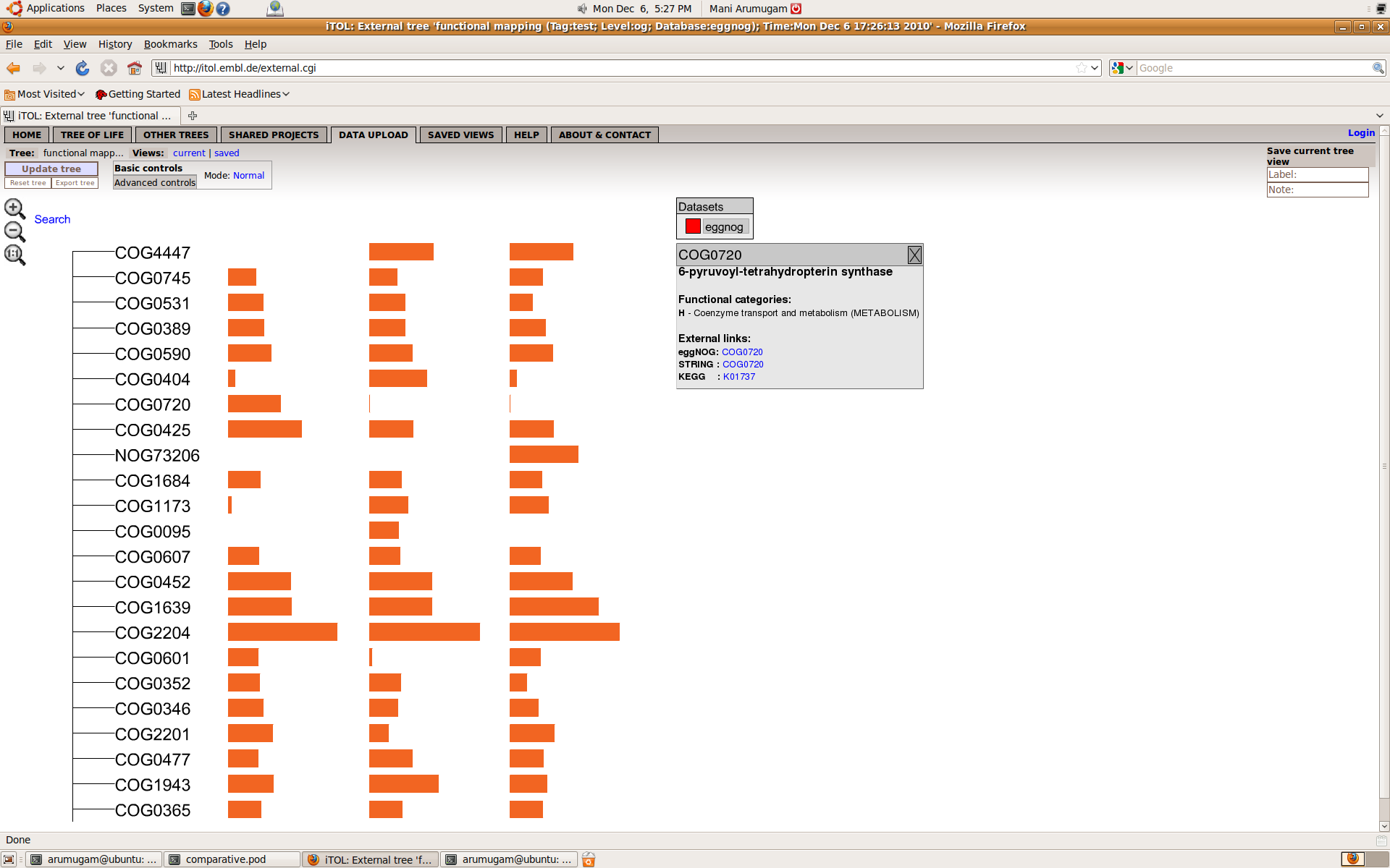
        doComparativeAnalysis.pl --analysis=functional --list=list.txt \
                --refdb=eggnog --tag=trial1 \
                --level=og --normalize=hits \
                --mode=itol
Since iTOL can display a lot of useful information on demand, this is a nice way of getting a first look at the data. If you thought iTOL is a tree-of-life viewer, you are wrong! Check out all the extra features it has at http://itol.embl.de. For the functional composition of a sample, iTOL will create a tree with one root and each functional group as a direct child of the root. However, you need to be careful because of the following reasons:
- there are thousands of orthologous groups
- several of them are of low abundance, so you wouldnt see anything in the graph
So we recommend restricting the display to the top 50 or 100 OGs in each sample, and filter OGs that have a very low abundance. So the recommended version of the command will be:
        doComparativeAnalysis.pl --analysis=functional --list=list.txt \
                --refdb=eggnog --tag=trial1 \
                --level=og --normalize=hits \
                --top=50 --filterlow=0.0001 \
                --mode=itol
A successful run looks like this:
        Processing samples ... done
        Filtering samples ... done
        Running: /g/bork3/x64/bin/perl /g/bork3/home/arumugam/svn_workspace/Smash/bin//iTOL_upload
        er.pl --config trial1.functional.cfg
        ITOL:
        ITOL: iTOL batch uploader
        ITOL: ===================
        ITOL: Upload successful. Your tree is accessible using the following iTOL tree ID:
        ITOL:
        ITOL: 111111111111111111111111
        ITOL:
        Upload successful. You can view this tree on iTOL using this URL:
        http://itol.embl.de/external.cgi?tree=111111111111111111111111
        Running: /g/bork3/x64/bin/perl /g/bork3/home/arumugam/svn_workspace/Smash/bin//iTOL_downlo
        ader.pl --tree 111111111111111111111111 --format svg --outputFile trial1.functional.downl
        oaded.svg --fontSize 20 --displayMode normal --colorBranches 1 --alignLabels 1 --scaleFact
        or 1 --showBS 1 --BSdisplayValue M0 --BSdisplayType text --datasetList dataset1

        iTOL batch downloader
        =====================
        Exported tree saved to trial1.functional.downloaded.svg
        <output>success</output>
The script tells you the commands it is executing to upload and download the tree to iTOL. Lines beginning with
"ITOL:"are what it received as a response from iTOL webserver, for your information. When the upload is successful, you can view the tree following the link provided. Hovering your mouse over any bar will show the name of the dataset, and the abundance of the corresponding functional group in that dataset.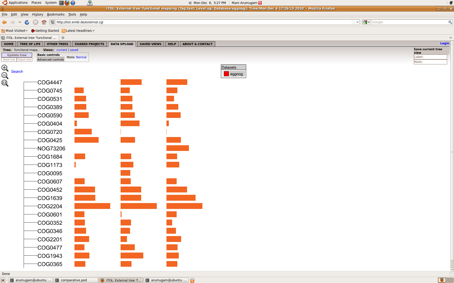
If you want to know more details about any of the orthologous groups, just move your mouse over it and iTOL will display, if available, the functional description, COG functional category, as well as links to eggNOG, STRING and KEGG websites.